2021. 1. 4. 12:52ㆍ머신러닝 교과서 with 파이썬, 사이킷런, 텐서플로
선형 SVM과 회귀분석과 같은 알고리즘은 비선형으로 구별되는 클래스를 구분 짓지 못한다.

이때 매핑함수\(\phi\)를 활용한 커널 방식을 사용한다면 비선형 문제를 해결할 수 있다.
매핑 함수를 활용해 원본 특성의 비선형 조합을 선형적으로 구분되는 고차원 공간에 투영시키고 이 공간에서의 초평면을 구분한 뒤 다시 원본 특성 공간으로 돌리면 비선형 결정 경계를 구분 지을 수 있게 된다.
Ex) \(\phi(x_1,x_2) = (z_1,z_2,z_3) = (x_1,x_2,x_1^2+x_2^2)\)
'2차원 -> 3차원 -> 2차원'의 투영 과정을 통해 결정 경계를 정의할 수 있다.
다만 매핑 함수의 문제점은 새로운 특성을 만드는 계산 비용이 매우 비싸다는 점이다. 특히 고차원 데이터일 경우에는 계산 비용이 더 비싸진다. 이를 해결하기 위해 두 포인트 사이 점 곱으로 이루어진 커널 함수를 사용한다.
커널 함수 : \(K(x^{(i)}, x^{(i)}) = \phi(x^{(i)})^{T}\phi(x^{(j)})\)
가장 자주 사용되는 커널 중 하나는 방사 기저 함수(가우시안 커널)이다.
\(K(x^{(i)}, x^{(i)}) =exp\left(-\frac{||x^{(i)} - x^{(j)}||^2}{2\sigma^2}\right) = exp(-\gamma||x^{(i)} - x^{(j)}||^2)\)
* \(\gamma =\frac{1}{2\sigma^2}\)
\(\gamma\)는 가우시안 구의 크기를 제한하는 역할을 하는 파라미터이다. \(\gamma\)값이 증가하면 서포트 벡터의 영향과 범위가 줄어든다. 이에 따라 결정 경계는 샘플에 조금 더 가까워지고 구불구불해진다.
커널이라는 용어는 샘플 간의 유사도 함수로 해석할 수도 있다. 음수 부호가 거리 측정을 유사도 점수로 바꾸는 역할을 한다. 지수 함수를 통해 얻게 되는 유사도 점수는 1과 0 사이의 값을 얻게 된다.
SVM을 활용한 비선형 문제 해결하기
라이브러리 불러오기
import numpy as np
import matplotlib.pyplot as plt
from matplotlib.colors import ListedColormap

from sklearn.svm import SVC
from sklearn import datasets
from sklearn.model_selection import train_test_split
from sklearn.preprocessing import StandardScaler
비선형 데이터 생성하기
np.random.seed(1)

# Create nonlinear dataset
X_xor = np.random.randn(200, 2)
y_xor = np.logical_xor(X_xor[:, 0] > 0,
                      X_xor[:, 1] > 0)
y_xor = np.where(y_xor, 1, -1)
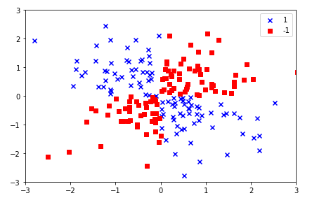
산점도 그래프 그려보기
# scatter plot
plt.scatter(X_xor[y_xor == 1, 0],
           X_xor[y_xor == 1, 1],
           c = 'b', marker = 'x',
           label = '1')
plt.scatter(X_xor[y_xor == -1, 0],
           X_xor[y_xor == -1, 1],
           c = 'r', marker = 's',
           label = '-1')
plt.xlim([-3, 3])
plt.ylim([-3, 3])
plt.legend(loc = 'best')
plt.tight_layout()
plt.show()
결정 경계 그래프 함수 만들기
# define function about visualizing decision_regions
def plot_decision_regions(X, y, classifier, test_idx = None, resolution = 0.02):

    # set marker and colormap
    markers = ('s', 'x', 'o', '^', 'v')
    colors = ('red', 'blue', 'lightgreen', 'cyan')
    cmap = ListedColormap(colors[:len(np.unique(y))])

    # draws a decision boundary.
    x1_min, x1_max = X[:, 0].min() - 1, X[:, 0].max() + 1
    x2_min, x2_max = X[:, 1].min() - 1, X[:, 1].max() + 1
    xx1, xx2 = np.meshgrid(np.arange(x1_min, x1_max, resolution),
                          np.arange(x2_min, x2_max, resolution))
    Z = classifier.predict(np.array([xx1.ravel(), xx2.ravel()]).T)
    Z = Z.reshape(xx1.shape)
    plt.contourf(xx1, xx2, Z, alpha = 0.3, cmap = cmap)
    plt.xlim(xx1.min(), xx1.max())
    plt.ylim(xx2.min(), xx2.max())

    for idx, cl in enumerate(np.unique(y)):
        plt.scatter(X[y == cl, 0], X[y == cl, 1],
                   alpha = 0.8, c = colors[idx],    # alpha : size of marker
                   marker = markers[idx], label = cl,
                   edgecolor = 'black')

    if test_idx:
        X_test, y_test = X[test_idx, :], y[test_idx]

        plt.scatter(X_test[:, 0], X_test[:, 1],
                   c = '', edgecolor = 'black', alpha = 1,
                   s = 100, label = 'test set')
모델링 학습 및 결정경계 확인
svm = SVC(kernel = 'rbf', random_state = 1, gamma = 0.1, C = 10)
svm.fit(X_xor, y_xor)
plot_decision_regions(X_xor, y_xor, classifier = svm)
plt.legend(loc = 'upper left')
plt.tight_layout()
plt.show()
비선형적으로 결정 경계가 형성된 것을 확인할 수 있다.
선형적으로 구분이 가능한 데이터도 결정 경계를 선형과 유사하게 바꿔 문제를 해결할 수 있다.

'머신러닝 교과서 with 파이썬, 사이킷런, 텐서플로' 카테고리의 다른 글
| [7] 랜덤 포레스트에 대해서 (0) | 2021.01.07 |
|---|---|
| [6] 의사결정나무의 정보이득과 불순도 (0) | 2021.01.06 |
| [4] 서포트 벡터 머신(SVM) 원리 이해하기 (선형) (0) | 2020.12.31 |
| [3] 로지스틱 회귀분석 원리 (0) | 2020.12.31 |
| [2] 아달린(Adaline, 적응형 선형 뉴런) 구현해보기 (0) | 2020.12.31 |