2021. 1. 4. 14:05ㆍEnglish/Machine learning algorithm
Algorithms such as linear SVMs and regression cannot distinguish classes that are distinguished by nonlinearity.


Using kernel methods using the mapping function\(\phi\) can solve nonlinear problems.
Using the mapping function, the nonlinear combination of the original characteristics can be projected into a linearly differentiated high-dimensional space, where the hyperplane is distinguished and then turned back into the original characteristic space to distinguish nonlinear decision regions.
Ex) \(\phi(x_1,x_2) = (z_1,z_2,z_3) = (x_1,x_2,x_1^2+x_2^2)\)
Decision regions can be defined by a projection process of '2D -> 3D -> 2D'.
However, the problem with mapping functions is that the computational cost of creating new characteristics is very expensive. Calculation costs become more expensive, especially for high-dimensional data. To solve this problem, we use a kernel function consisting of dots between two points.
kernel function : \(K(x^{(i)}, x^{(i)}) = \phi(x^{(i)})^{T}\phi(x^{(j)})\)
One of the most frequently used kernels is the radiation base function (Gaussian kernel).
\(K(x^{(i)}, x^{(i)}) =exp\left(-\frac{||x^{(i)} - x^{(j)}||^2}{2\sigma^2}\right) = exp(-\gamma||x^{(i)} - x^{(j)}||^2)\)
* \(\gamma =\frac{1}{2\sigma^2}\)
\(\gamma\) is a parameter that serves to limit the size of the Gaussian sphere. Increasing the \(\gamma\) value reduces the influence and scope of the support vector. As a result, the decision regions become a little closer to the sample and more winding.
The term kernel can also be interpreted as a similarity function between samples. Negative signs translate distance measurements into similarity scores. The similarity score obtained through the exponential function will be between 1 and 0.
Using SVM to solve nonlinear problems
Load Library
import numpy as np
import matplotlib.pyplot as plt
from matplotlib.colors import ListedColormap

from sklearn.svm import SVC
from sklearn import datasets
from sklearn.model_selection import train_test_split
from sklearn.preprocessing import StandardScaler
Create non-linear data
np.random.seed(1)

# Create nonlinear dataset
X_xor = np.random.randn(200, 2)
y_xor = np.logical_xor(X_xor[:, 0] > 0,
                      X_xor[:, 1] > 0)
y_xor = np.where(y_xor, 1, -1)
Draw scatter plot graphs
# scatter plot
plt.scatter(X_xor[y_xor == 1, 0],
           X_xor[y_xor == 1, 1],
           c = 'b', marker = 'x',
           label = '1')
plt.scatter(X_xor[y_xor == -1, 0],
           X_xor[y_xor == -1, 1],
           c = 'r', marker = 's',
           label = '-1')
plt.xlim([-3, 3])
plt.ylim([-3, 3])
plt.legend(loc = 'best')
plt.tight_layout()
plt.show()
Create Decision Regions Graph Function
# define function about visualizing decision_regions
def plot_decision_regions(X, y, classifier, test_idx = None, resolution = 0.02):

    # set marker and colormap
    markers = ('s', 'x', 'o', '^', 'v')
    colors = ('red', 'blue', 'lightgreen', 'cyan')
    cmap = ListedColormap(colors[:len(np.unique(y))])

    # draws a decision boundary.
    x1_min, x1_max = X[:, 0].min() - 1, X[:, 0].max() + 1
    x2_min, x2_max = X[:, 1].min() - 1, X[:, 1].max() + 1
    xx1, xx2 = np.meshgrid(np.arange(x1_min, x1_max, resolution),
                          np.arange(x2_min, x2_max, resolution))
    Z = classifier.predict(np.array([xx1.ravel(), xx2.ravel()]).T)
    Z = Z.reshape(xx1.shape)
    plt.contourf(xx1, xx2, Z, alpha = 0.3, cmap = cmap)
    plt.xlim(xx1.min(), xx1.max())
    plt.ylim(xx2.min(), xx2.max())

    for idx, cl in enumerate(np.unique(y)):
        plt.scatter(X[y == cl, 0], X[y == cl, 1],
                   alpha = 0.8, c = colors[idx],    # alpha : size of marker
                   marker = markers[idx], label = cl,
                   edgecolor = 'black')

    if test_idx:
        X_test, y_test = X[test_idx, :], y[test_idx]

        plt.scatter(X_test[:, 0], X_test[:, 1],
                   c = '', edgecolor = 'black', alpha = 1,
                   s = 100, label = 'test set')
Learn modeling and identify decision regions
svm = SVC(kernel = 'rbf', random_state = 1, gamma = 0.1, C = 10)
svm.fit(X_xor, y_xor)
plot_decision_regions(X_xor, y_xor, classifier = svm)
plt.legend(loc = 'upper left')
plt.tight_layout()
plt.show()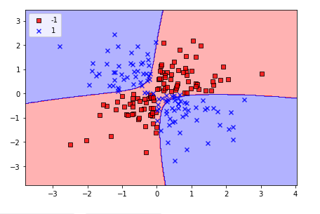
We can confirm the formation of decision regions nonlinearly.
Linearly separable data can also solve the problem by changing the decision regions to resemble the linear ones.

'English > Machine learning algorithm' 카테고리의 다른 글
| [7] About RandomForest (0) | 2021.01.07 |
|---|---|
| [6] Information gain and impurity of decision tree (0) | 2021.01.06 |
| [4] Understand Support Vector Machine (SVM) Principles (linear) (0) | 2020.12.31 |
| [3] Logistic Regression Principles (0) | 2020.12.31 |
| [2] Implement Adaline (adaptive linear neuron) (0) | 2020.12.31 |