2020. 12. 31. 18:15ㆍEnglish/Machine learning algorithm
This post is code from notbook, which won bronze medal in kaggle. If you are interested, please refer to the laptop.
www.kaggle.com/choihanbin/predict-titanic-survival-by-adaptive-linear-neuron
In the previous posting, we looked at perceptron. This time we're going to talk about Adalin, a slightly modified version of this.
2020/12/31 - [English/Machine learning algorithm] - [1] Try implementing Perceptron
What is Adalin?
Adalin stands for Adaptive linear neuron. Adaptive linear neurons can be thought of as an improved version of the perceptron. The biggest relationship with the perceptron is to use the linear activation function instead of the unit step function, such as the perceptron, to update weights. This has the advantage of being differentiable in cost functions. This allows us to find weights that minimize the cost function. We will use the gradient descent method as an optimization algorithm to implement it.
Concept of gradient descent
Gradient descent is a method that differentiates a cost function that can be defined as a convex function and allows you to find a global minimum. If you think simply, you can use differentiation to find the minimum value of the cost function. You mentioned above that adaptive linear neurons utilize linear activation functions, right? You may wonder why you need to put a linear function (f(x) = x), but that's because of the advantage of being differentiable. Differentiation makes it easy to find the minimum value of the cost function.
Adalin's Weighted Learning Rules
The weight change (\(\Delta w\)) is defined as the negative gradient multiplied by the learning rate \(\eta \).
$$ \Delta w = -\eta▽J(w)$$
To get the gradient \(\delta\) J(w) of the cost function here, you need to calculate a one-way function for each weight \(w_j\).
$$ \frac {\delta J}{\delta w_j} = -sum_i(y^{(i)} - \phi(z^{(i)}))x^{(i)}$$
As a result, you can write the update formula for weight \(w_j\) as follows:
$$ \Delta w = \eta\sum_i(y^{(i)} - \phi(z^{(i)}))x^{(i)}$$
Technically speaking, the above method is to apply the batch gradient descent method.
Batch gradient descent vs. Stochastic gradient descent
How the weights are updated determines how the gradient descent is done. If you update weights based on all samples in the training set, they are called batch gradient descent. So it's not the same way that the perceptron in the previous posting updated the weights for each sample.
$$ \Delta w = \eta\sum_i(y^{(i)} - \phi(z^{(i)}))x^{(i)} $$
Update Weight of Batch Gradient Descent Method
* \(\eta \) : Learning rate
But if you use that method for a very large data set, it's going to be very expensive. To compensate for this, we use a method called stochastic gradient descent. This is to update the weights little by little for each training sample. However, when using this, it is very important to randomly input the training samples, and it is important to mix them so that they are not injected in the same order for each epoch. This can be used as online learning because each training sample can be learned.
$$ \Delta w = \eta(y^{(i)} - \phi(z^{(i)}))x^{(i)} $$
Update Weight of Stochastic Gradient Descent Method
And then there's mini-batch learning that compromises these two. This applies batch gradient descent to a small fraction of the training data. The weight update is faster to converge the weights than the batch gradient descent.
Let's see how Adalin can be implemented under these learning rules.
Implementation
Load the required library.
import numpy as np
import pandas as pd
import matplotlib.pyplot as plt
%matplotlib inline

import warnings
warnings.filterwarnings('ignore')

from sklearn.preprocessing import StandardScaler
Load the data
train = pd.read_csv('../input/titanic/train.csv')
test = pd.read_csv('../input/titanic/test.csv')
train.head()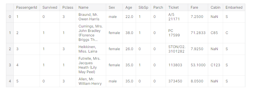
Adjust the feature.
(feature engineering was conducted based on https://www.kaggle.com/choihanbin/titanic-survival-prediction-eda-ensemble. This is not important in the Adalin implementation, so we'll move on.)
# concate dataset(train, test)
df = pd.concat(objs = [train, test], axis = 0).reset_index(drop = True)

# fill null-values in Age
age_by_pclass_sex = df.groupby(['Sex', 'Pclass'])['Age'].median()
df['Age'] = df.groupby(['Sex', 'Pclass'])['Age'].apply(lambda x: x.fillna(x.median()))

# create Cabin_Initial feature
df['Cabin_Initial'] = df['Cabin'].apply(lambda s: s[0] if pd.notnull(s) else 'M')
df['Cabin_Initial'] = df['Cabin_Initial'].replace(['A', 'B', 'C', 'T'], 'ABCT')
df['Cabin_Initial'] = df['Cabin_Initial'].replace(['D', 'E'], 'DE')
df['Cabin_Initial'] = df['Cabin_Initial'].replace(['F', 'G'], 'FG')
df['Cabin_Initial'].value_counts()

# fill null-values in Embarked
df['Embarked'] = df['Embarked'].fillna('S')

# fill null-values in Fare
df['Fare'] = df['Fare'].fillna(df.groupby(['Pclass', 'Embarked'])['Fare'].median()[3]['S'])


# binding function for Age and Fare
def binding_band(column, binnum):
    df[column + '_band'] = pd.qcut(df[column].map(int), binnum)

    for i in range(len(df[column + '_band'].value_counts().index)):
        print('{}_band {} :'.format(column, i), df[column + '_band'].value_counts().index.sort_values(ascending = True)[i])
        df[column + '_band'] = df[column + '_band'].replace(df[column + '_band'].value_counts().index.sort_values(ascending = True)[i], int(i))

    df[column + '_band'] = df[column + '_band'].astype(int)

    return df.head()

binding_band('Age',8)
binding_band('Fare', 6)


# create Initial feature
df['Initial'] = 0
for i in range(len(df['Name'])):
    df['Initial'].iloc[i] = df['Name'][i].split(',')[1].split('.')[0].strip()

Mrs_Miss_Master = []
Others = []

for i in range(len(df.groupby('Initial')['Survived'].mean().index)):
    if df.groupby('Initial')['Survived'].mean()[i] > 0.5:
        Mrs_Miss_Master.append(df.groupby('Initial')['Survived'].mean().index[i])
    elif df.groupby('Initial')['Survived'].mean().index[i] != 'Mr':
        Others.append(df.groupby('Initial')['Survived'].mean().index[i])

df['Initial'] = df['Initial'].replace(Mrs_Miss_Master, 'Mrs/Miss/Master')
df['Initial'] = df['Initial'].replace(Others, 'Others')

# create Alone feature
df['Alone'] = 0
df['Alone'].loc[(df['SibSp'] + df['Parch']) == 0] = 1

# create Companinon's survival rate feature
df['Ticket_Number'] = df['Ticket'].replace(df['Ticket'].value_counts().index, df['Ticket'].value_counts())
df['Family_Size'] = df['Parch'] + df['SibSp'] + 1
df['Companion_Survival_Rate'] = 0
for i, j in df.groupby(['Family_Size', 'Ticket_Number'])['Survived'].mean().index:
    df['Companion_Survival_Rate'].loc[(df['Family_Size'] == i) & (df['Ticket_Number'] == j)] = df.groupby(['Family_Size', 'Ticket_Number'])["Survived"].mean()[i, j]

comb_sum = df.loc[df['Family_Size'] == 5]['Survived'].sum() + df.loc[df['Ticket_Number'] == 3]['Survived'].sum()
comb_counts = df.loc[df['Family_Size'] == 5]['Survived'].count() + df.loc[df['Ticket_Number'] == 3]['Survived'].count()
mean = comb_sum / comb_counts

df['Companion_Survival_Rate'] = df['Companion_Survival_Rate'].fillna(mean)

# select categorical features
cate_col = []
for i in [4, 11, 12, 15]:
    cate_col.append(df.columns[i])

cate_df = pd.get_dummies(df.loc[:,(cate_col)], drop_first = True)
df = pd.concat(objs = [df, cate_df], axis = 1).reset_index(drop = True)

df = df.drop(['Name', 'Sex', 'Age', 'Ticket', 'Fare', 'Embarked', 'Cabin_Initial', 'SibSp', 'Parch',
              'Cabin', 'Initial', 'Ticket_Number', 'Family_Size'], axis = 1)

# split data
df = df.astype(float)
train = df[:891]
test = df[891:]

train_X = StandardScaler().fit_transform(train.drop(columns = ['PassengerId', 'Survived']))
train_y = train.iloc[:, 1]
test_X = StandardScaler().fit_transform(test.drop(columns = ['PassengerId', 'Survived']))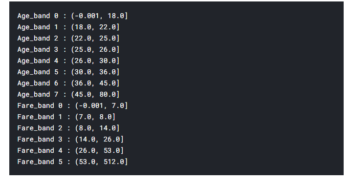
Adalin implementation using batch gradient descent
class AdalineBGD(object):
    def __init__(self, eta = 0.01, n_iter = 50, random_state = 1):
        self.eta = eta
        self.n_iter = n_iter
        self.random_state = random_state

    def fit(self, X, y):
        rgen = np.random.RandomState(self.random_state)
        self.w_ = rgen.normal(loc = 0, scale = 0.01,
                             size = 1 + X.shape[1])
        self.cost_ = []

        for i in range(self.n_iter):
            net_input = self.net_input(X)
            output = self.activation(net_input)
            errors = (y - output)
            self.w_[1:] += self.eta * X.T.dot(errors)
            self.w_[0] += self.eta * errors.sum()
            cost = (errors**2).sum() / 2
            self.cost_.append(cost)
        return self

    def net_input(self, X):
        return np.dot(X, self.w_[1:]) + self.w_[0]

    def activation(self, X):
        return X

    def predict(self, X):
        return np.where(self.activation(self.net_input(X)) >= 0, 1, 0)
What's different about the previously implemented perceptron framework is that the activation function and the way the weights are updated and the cost function is calculated.
Cost graph based on learning rate
fig, ax = plt.subplots(1, 2, figsize = (10, 4))
PCbgd1 = AdalineBGD(eta = 0.01, n_iter = 10)
PCbgd1.fit(train_X, train_y)
ax[0].plot(range(1, len(PCbgd1.cost_) + 1),
          np.log10(PCbgd1.cost_), marker = 'o')
ax[0].set_xlabel('Epochs')
ax[0].set_ylabel('log(SSE)')
ax[0].set_title('Adaline - learning rate 0.01')

PCbgd2 = AdalineBGD(eta = 0.0001, n_iter = 10)
PCbgd2.fit(train_X, train_y)
ax[1].plot(range(1, len(PCbgd2.cost_) + 1),
          np.log10(PCbgd2.cost_), marker = 'o')
ax[1].set_xlabel('Epochs')
ax[1].set_ylabel('log(SSE)')
ax[1].set_title('Adaline - Learning rate 0.0001')
plt.show()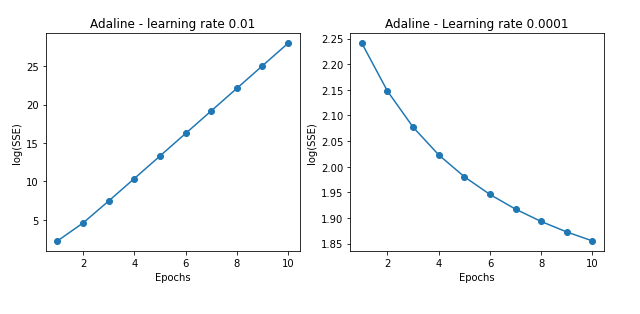
When the learning rate is 0.01, it's so large that you can see that the cost increases gradually as you go through the global sea and progress through the learning process. On the other hand, when the learning rate is 0.0001, you can see that the learning rate is too small to reach the discharge year.
fig, ax = plt.subplots(figsize = (15, 6))
PCbgd3 = AdalineBGD(eta = 0.0005, n_iter = 10)
PCbgd3.fit(train_X, train_y)
ax.plot(range(1, len(PCbgd3.cost_) + 1),
          np.log10(PCbgd3.cost_), marker = 'o')
ax.set_xlabel('Epochs')
ax.set_ylabel('log(SSE)')
ax.set_title('Adaline - Learning rate 0.0001')
plt.show()
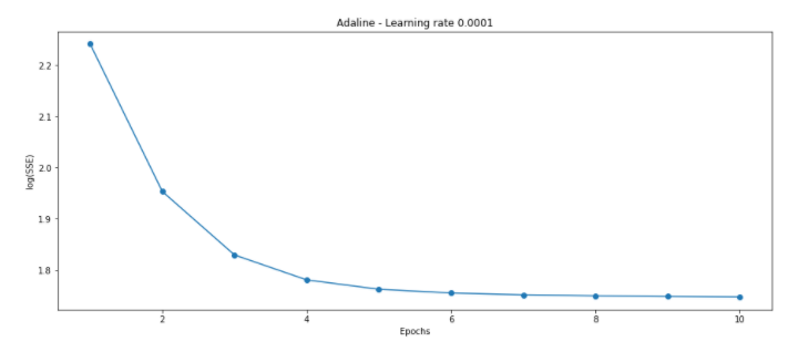
The appropriate learning rate and epochs were found.
Adalin implementation using stochastic gradient descent
class AdalineSGD(object):
	def __init__(self, eta = 0.1, n_iter = 10,
                shuffle = True, random_state = None):
        self.eta = eta
        self.n_iter = n_iter
        self.w_initialized = False
        self.shuffle = shuffle
        self.random_state = random_state

    def fit(self, X, y):
        self._initialize_weights(X.shape[1])
        self.cost_ = []

        for i in range(self.n_iter):
            if self.shuffle:
                X, y = self._shuffle(X, y)
            cost = []
            for xi, target in zip(X, y):
                cost.append(self._update_weight(xi, target))
            avg_cost = sum(cost) / len(y)
            self.cost_.append(avg_cost)
        return self

    def partial_fit(self, X, y):
        # train data not reset weights
        if not self.w_initialized:
            self._initialize_weight(X.shape[1])
        if y.ravel().shape[0] > 1:
            for xi, target in zip(X, y):
                self._update_weight(xi, target)
        else:
            self._update_weight(X, y)
        return self

    def _shuffle(self, X, y):
        r = self.rgen.permutation(len(y))
        return X[r], y[r]

    def _initialize_weights(self, m):
        self.rgen = np.random.RandomState(self.random_state)
        self.w_ = self.rgen.normal(loc = 0, scale = 0.01,
                                  size = 1 + m)
        self.w_initialized = True

    def _update_weight(self, xi, target):
        output = self.activation(self.net_input(xi))
        error = (target - output)
        self.w_[1:] += self.eta * xi.dot(error)
        self.w_[0] += self.eta * error
        cost = (error**2) / 2
        return cost

    def net_input(self, X):
        return np.dot(X, self.w_[1:]) + self.w_[0]

    def activation(self, X):
        return X

    def predict(self, X):
        return np.where(self.activation(self.net_input(X)) >= 0, 1, 0)
It looks a little complicated. This is because they made it possible to implement additional learning data in an already created model, even if they were given additional learning data. You can see that the way weights are updated is different from batch gradient descent. As I explained above, we added a function called 'shuffle' to randomly mix the order of the training samples so that each fork has a different order.
Cost graph based on learning rate
fig, ax = plt.subplots(1, 2, figsize = (10, 4))

for i, eta in enumerate([0.05, 0.0001]):
    AD = AdalineSGD(eta = eta, n_iter = 10)
    AD.fit(train_X, train_y)
    ax[i].plot(range(1, len(AD.cost_) + 1),
              np.log10(AD.cost_), marker = 'o')
    ax[i].set_title('Adaline - Learing rate {}'.format(eta))
    ax[i].set_xlabel('Epochs')
    ax[i].set_ylabel('Log(SSE)')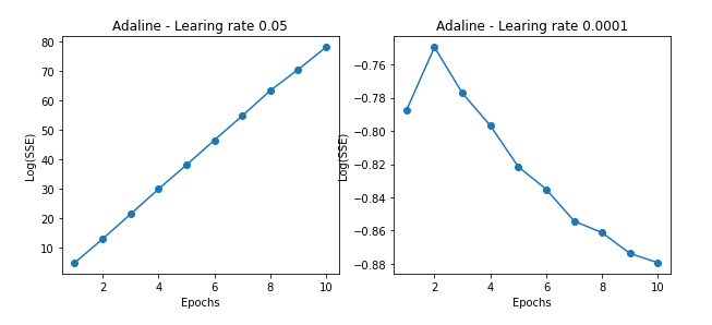
fig, ax = plt.subplots(figsize = (15, 6))
ADsgd = AdalineSGD(eta = 0.005, n_iter = 10)
ADsgd.fit(train_X, train_y)
ax.plot(range(1, len(PCbgd3.cost_) + 1),
          np.log10(PCbgd3.cost_), marker = 'o')
ax.set_xlabel('Epochs')
ax.set_ylabel('log(SSE)')
ax.set_title('Adaline - Learning rate 0.005')
plt.show()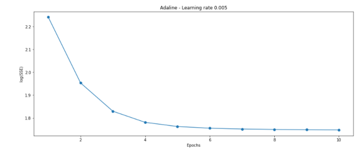
For each model, the appropriate learning rate and epoch were selected and submitted to the kagle reader board, which was *less than expected.
* batch gradient descent : 0.65550
* stochastic gradient descent : 0.69617
This seems to be because Adalin model does not fit the data set.
In the next posting, we will look at logistic regression.
'English > Machine learning algorithm' 카테고리의 다른 글
| [6] Information gain and impurity of decision tree (0) | 2021.01.06 |
|---|---|
| [5] Non-linear Troubleshooting with Kernel SVM (0) | 2021.01.04 |
| [4] Understand Support Vector Machine (SVM) Principles (linear) (0) | 2020.12.31 |
| [3] Logistic Regression Principles (0) | 2020.12.31 |
| [1] Try implementing Perceptron (0) | 2020.12.31 |